Procedural generation using Quantum annealers
Disclaimer
You can find the io page here. This is a WIP. Updates coming soon are
1) Cool pictures to convey concepts easier
2) Actual generated maps
Introduction
You do not need a particularly extensive understanding of WFC to read this, but many of the choices here may not seem particularly interesting without the context of the “original” algorithm and its history. I am going to assume that the reader is either:
1) already fmailiar with Wave Function Collapse (WFC) to a degree
2) that they have read through the blog post linked here.
If the reader would like, a brief overview is provided below:
WFC Algorithm Overview
The following is a visual illustration of traditional WFC for procedurally generating a video game map. In this example we will use the a set of 16 tiles to fill a 2 by 2 space:
.png)
We start by choosing an empty map space we want to fill. We then select a tile at random from the list of possible legal tiles and place it down.
A tile can only be placed next to a tile with matching conections. As such, the two neighboring space have their list of possible tiles restricted. Since an empty and *unrestricted* space could be any of the 16 possible tiles it means we are very _uncertain_ of what will go there. Conversely, the two highlighted regions can now only be 1 of 8 pssible tiles meaning we are *more* certain of what will go there.
Of the three empty spaces we choose the region with the _greatest certainty_ to place a tile in. In the case of a tie we choose randomly amongst the tied spaces.
This process repeats. We asses how the placed tile affects the possiblities of adjacent spaces and choose the space with the greatest certainty.
Then randomly select a legal tile to place.
And repeat until the map is filled!
This is the core of how WFC procedurally generates maps. With just this you can build _correct_ maps, but you cannot guarantee building _interesting_ maps. Augmenting the algorithm is what controls the stylistic elements of the generated map. For instance controlling the probability of certain tile choices can result in concetric maps or dense mazes.
Disclaimer and overview aside, let’s overcomplicate an otherwise very simple and user-friendly algorithm using quantum computing.
Quickly though, why are we doing this at all?
The truth is that I’m a huge math nerd. The practical answer is to illustrate the unique properties of quantum computers—how they’re not simply faster than today’s computers, but solve optimization problems essentially unsolvable otherwise in milliseconds.
If a problem can be “realistically” converted into a form ingestible by a quantum computer, and you have the resources, then it likely should be. Unlike non-quantum solutions, the GLOBAL MINIMUM is found, an incredible guarantee in the realm of optimization. The disclaimer “realistically” has a lot of important factors we’ll talk about later. Before that, however, we need to explain an idea called Quadratic Unconstrined Binary Optimization (QUBO). Then we can discuss how QUBOs are used to solve problems leveraging quantum hardware. Finally, we can lay out how to take WFC and convert it into a QUBO problem to be solved on said hardware.
QUBO
Quadratic Unconstrained Binary Optimization (QUBO) is a mathematical formulation for Binary Optimization problems, or problems where each variable is binary (0 or 1). We want to find some optimal combination of these variables. A QUBO problem takes the form of:
\[y = x_1^2a_{1} + x_2^2a_{2} + x_3^2a_{3} … x_N^2a_{N} + 2x_1x_2a_{12} + …\]Where \(x_i\) are binary variables, \(a_{ij}\) is a set of weights for each choice, and \(y\) is the output we are trying to maximize or minimize. In a concrete example we can look at a scenario where we are want to buy the best snack food for a party within a budget:
| Item | Cost |
|---|---|
| \(x_{soda}\) | \(a_1=\)$4 |
| \(x_{chips}\) | \(a_2=\)$5 |
| \(x_{fruits}\) | \(a_3=\)$2 |
Given these items and cost, the binary formula for how much money we spend is:
\[Y = x_{soda}a_1 + x_{chips}a_2 + x_{fruits}a_3\]If \(x_i\) is a binary variable for “did we buy this item”, and \(a_i\) is the cost, then Y is the total dollar amount spent. Accounting for our budget B we can write out the difference between money spent and the budget as:
\[Budget = {\$9}\] \[Diff = ( \sum_{i=1}^3x_ia_i - B )^2\]By minimizing the difference we find the optimal combination of items to buy that brings us as close to our budget as possible. This is clearly the Soda and Chips since they total $9, but we could easily include every item in the grocery store’s inventory as a variable and find the optimal combination. To do that however we need to convert the difference equation into a QUBO, whcih takes the form:
This is our QUBO Equation from before, represented in matrix form. The goal is to find what combination of binary variables (0 or 1) will yield the optimal output y (either the minimum or maximum value). Funny enough, our contrived snack example is an optimization problem built up from binary decision variables! This can be converted into a QUBO—but first we need to write it out as a quadratic equation.
\[Diff = ( \sum_{i=1}^{N=3}x_ia_i - B )^2\]Writing out the sum gives:
\[Diff = ( x_1a_1 + x_2a_2 + x_3a_3 - B )^2\]Which expands to:
\[Diff = ( x_1a_1 + x_2a_2 + x_3a_3 - B ) * ( x_1a_1 + x_2a_2 + x_3a_3 - B )\]After factoring and writing back into summation form yields:
\[Diff = \sum_{i=1}^{N=3}\sum_{k=1}^{N=3}x_ia_ix_ka_k - 2\sum_{i=1}^{N=3}x_ia_iB + B^2\]Which should look similar to the quadratic equation
\[y = ax^2 + bx + c\]Now we can see the QUBO equation shown earlier ( \(y = xQx’\) ) has only second order terms, or terms raised to the power 2. Fortunately binary variables have a unique quality where a variable is equal to its square i.e \(1 = 1x1\) and \(0 = 0x0\). Therefore, \(x = x^2\). In our binary quadratic equation we will square each first order term making \(x_i = x_i^2\). Lastly, since we are solving an optimiation problem we are looking for some maximum or minimum on a curve. This max/min is independant from the constant term B in the problem. We can drop them resulting in:
\[Diff = \sum_{i=1}^{N=3}x_i^2(a_i^2 - 2a_iB) + 2\sum_{i=1}^{N=3}\sum_{k}x_ia_ix_ka_k\]Which can be written in matrix form as
\[Diff = xQx'\]Here, x is a vector of length 3 with a binary variable corresponding to buying a given snack. Q is a square matrix of size [3x3] with the self interaction coefficients (diagonal terms) \((a_i^2 - 2a_iB)\) and cross interaction coefficients (off diagonal terms) \(a_ia_k\). You can check that the vector x = [1, 1, 0] yields the minimum scalar output which corresponds to purchasing the Soda and Chips!
Reformulating this simple problem is likely a very silly over complication. Keep in mind: this method scales to multiple constraints! A great quality of QUBO is that the constraint matrix Q is additive with any other Q matrix of equal size. We could create a new optimization constraint, say, the flavor constraint \(Q_{flavor}\) so we equitably purchase a diverse range of party snack flavors and not just chips. We could then make a new QUBO formulation by adding the two Q matrices together. This means a QUBO problem can have a large number of constraints applied without increasing the memory usage of the problem itself (the number of variables).
A base assumption we’ll take, but not discuss in this article: we’ll assume QUBO problems are capable of being solved via quantum hardware. The how is equally interesting, but: 1) a digression from WFC as used for procedural generation in video games and 2) not something I am particularly qualified to explain. Suffice to say the benefits of QUBOs on quantum hardware are as follows:
1) A large combinatorial problem can be impossible to solve classically 2) The quantum solution is easily 1e4 times faster than classical techniques (like genetic algorithms). I have seen this in professional settings, and it gets faster. 3) It does this while finding the global minimum.
QUBO applied to procedural generation (WFC)
As it relates to procedural generation in video games, using WFC we have:
1) An empty grid map 2) A set of tiles we can place in each grid space 3) A set of adjacency rules dictating what tiles can be placed next to one another
How can we formulate this as a QUBO?
First, we define a set of binary variables that correspond to a decision to place a single tile type in a single map space. We will be using the following set of 16 tiles to generate a dungeon:
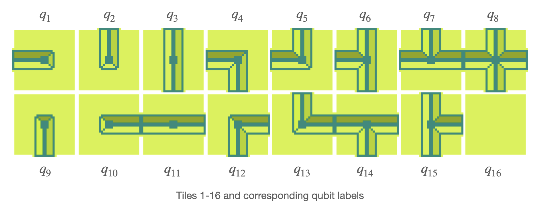
For each empty space in the map we are trying to decide which of these 16 tiles we want to place. We therefore assign a binary variable to each tile type for each map space. In this problem we will define the binary variable \(x_{i,j,k}\) as the decision to place type K placed at map coordinate [i,j]. In an [8x8] sized map with 16 tile types this yields 1024 binary variables.
On a standard computer a binary variable is represented by a bit. A quantum computer uses bits as well, but distinguishes them from traditional computers by calling them quantum bits (qubits). A qubit is different from a bit, and leverages quantum physics principles to do things I am unqualified to explain at the moment. For us to run our QUBO problem on a digital annealer we will assign a qubit to each of our 1024 binary variables. The annealer will return a binary vector whose qubits represent the solution to the optimization problem formed by the constraint matrix Q. To do this for WFC we need to develop 2 constraints:
1) We cannot place more than 1 tile per map coordinate 2) A tile can only be placed next to a valid neighboring tile
Without constraint [1] the annealer could activate multiple qubits per map coordinate i.e. telling us to place a water tile and wall tile in the same space. To prevent this we need a constraint that defines placing more than 1 tile per space as suboptimal (this is found under the oneHotQ function). Since the annealer will find the global minimum it will never output a solution that violates this constraint IF we formulate it correctly. Since we only want one qubit to activate per space we can write this constraint mathematically as:
\[\sum_{i}^Nx_i = 1\]For two variables we write the optimization equation as
\[E = ( 1 - x - y + 2xy )\]And for 3
\[E = ( 1 - x - y - z + 2xy + 2xz + 2yz )\]Etc. As you can see the cross interaction terms are +2 and the self interaction terms are -1. Since I have arbitrarily decided to write this as a maximization problem I swapped the signs making the Q matrix:
\[Q = \begin{bmatrix} 1 & -2 & -2 & ... & -2\\ -2 & 1 & -2 & ... & -2\\ -2 & -2 & 1 & ... & -2\\ & & ... & & \\ -2 & -2 & -2 & ... & 1 \end{bmatrix}\]
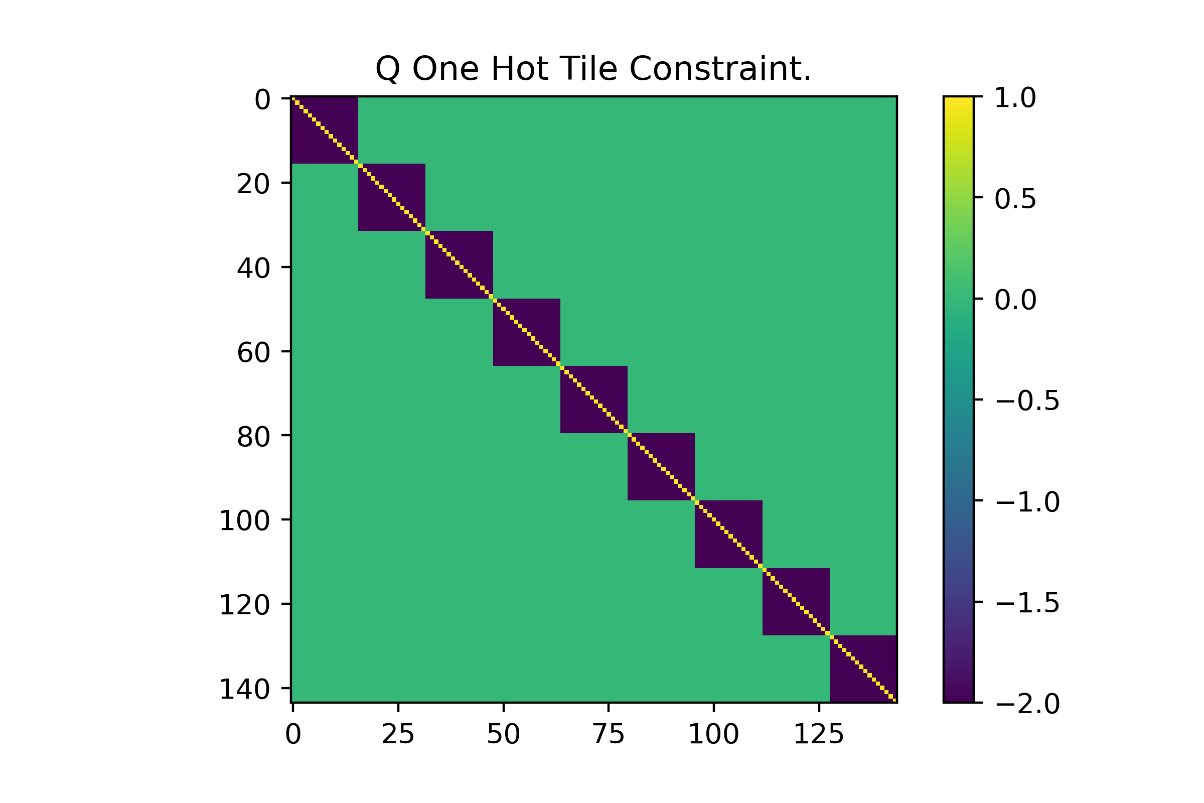
As you might see, by activating only 1 qubit we get an energy of 1. By activating any 2 qubits we get an energy of 0, any 3 = -4, etc… Since the annealer will find the globally optimal solution to our Q matrix it does not matter how close the optimal answer is to any sub-optimal answers. A visual of the Q matrix is shown below for our set of 16 tiles over a [3x3] map space. It is hard to tell since these matrices grow large very quickly, but this constraint only affects variables in increments of 16. This reflects how we are using 16 tiles per grid space. On a [3x3] map we have (3)(3)(16)=144 variables.
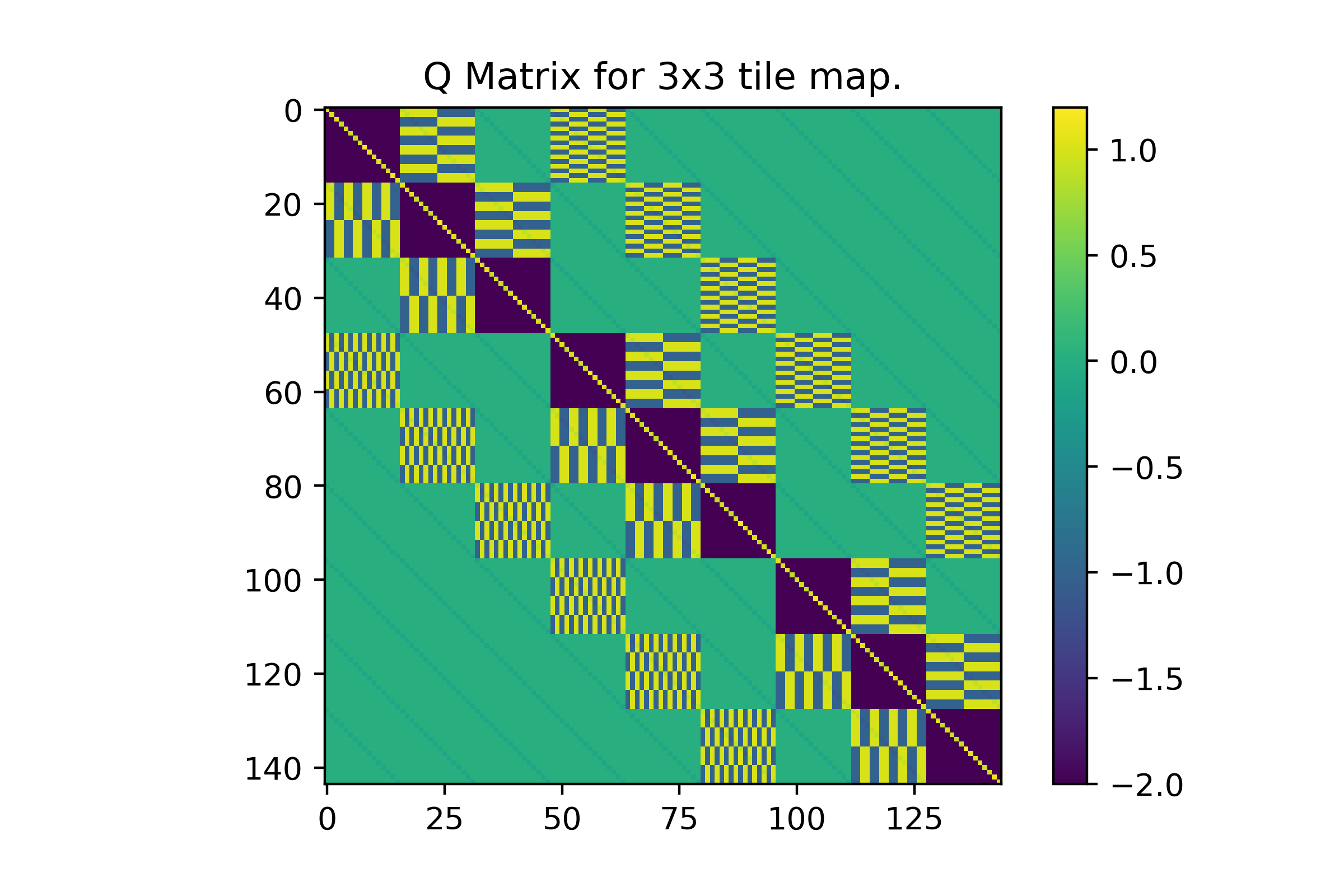
The second constraint (legal neighbor placement) is equally simple. For each tile type at a given map space [i,j] we need to reward the annealer for activating a neighboring qubit if and only if it is a legal tile placement. We should also penalize it if it’s an illegal combination (This is done in the genLegalQ function). To demonstrate, let the qubit \(x_{i,j,k}\) correspond to a tile type K placed at map coordinate [i,j]. Take as example the qubits \(x_{0,0,0}\) and \(x_{1,0,5}\). If it’s legal to place tile 5 above tile 0 then the cross coefficient \(a\) in \(ax_{0,0,0}x_{1,0,5}\) will be 1, and if it’s illegal it will be -1. A visual of this constraint is shown below.
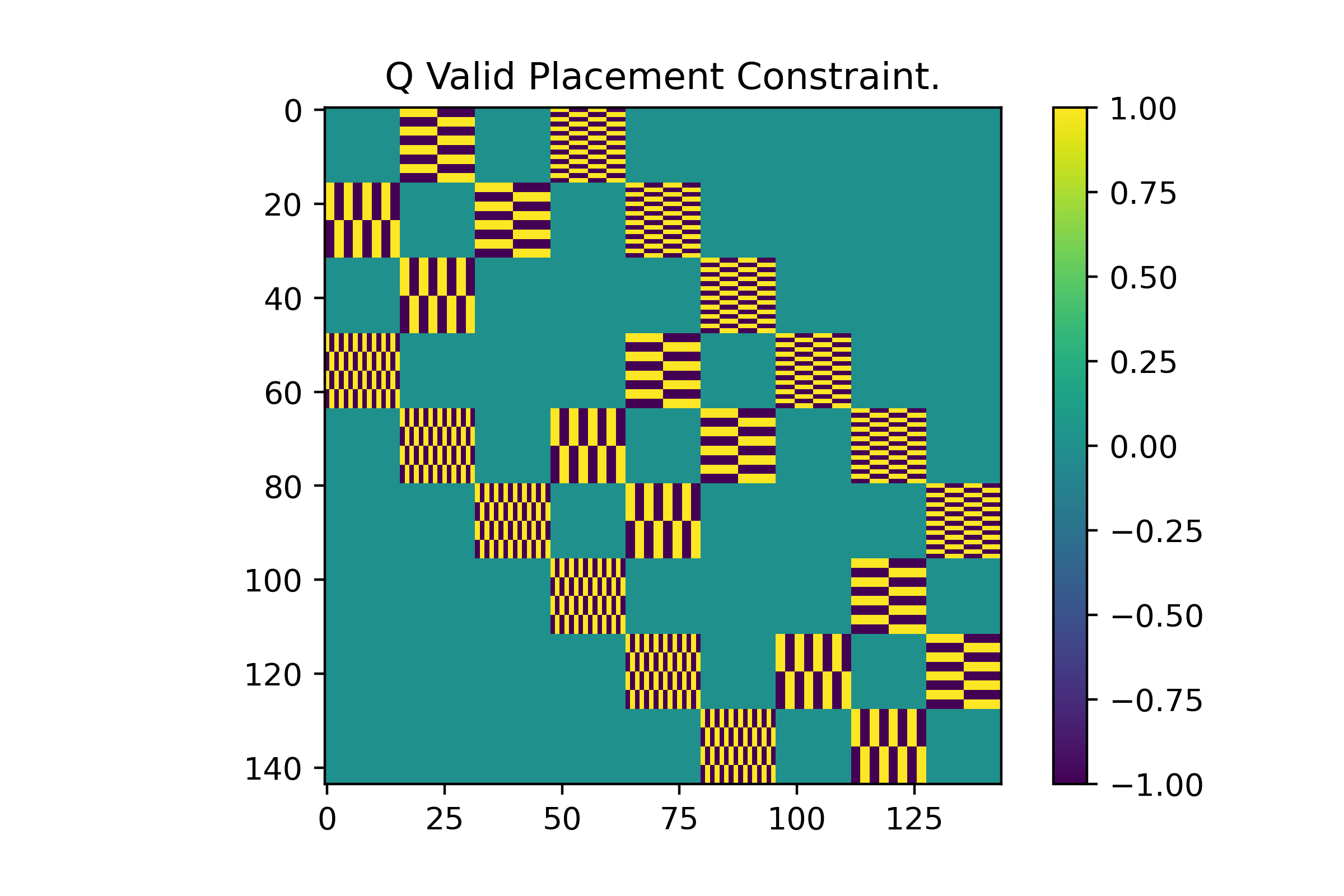
This is likely the most visually distinct of the constraints I will lay out here so I will dissect it a little more in detail. It should be apparent with this image that the Q matrix in a QUBO formulation is symmetric. Noting this, you can asses how a constraint affects the optimization problem by either looking at the columns or rows. To start lets focus on the map space [0,0] which corresponds to the first 16 variables. We can tell visually that this constraint only cares about the cross interaction terms since all interaction term weights within a tile space are set to 0 (i.e. weights between variables 0-16). The next thing we can tell is how many adjacent map spaces our chosen tile cares about (looking at either the row or column). In this case, the corner [0,0] only needs to ensure a legal placement with its NSEW neighbors [0,1] and [1,0]. As such we only have two regions where cross-interaction terms are non-zero, which are the sets of 16 variables assigned those two map spaces. The last thing to note is that we technically have 4 different cross-interaction patterns which may be more apparent along the rows roughly spanning 60 to 80. These are different because, for each tile, its legal placement changes depending on which location among NSEW it is placed.
The new Q matrix is comprised of both these constraints
\(Q = Q_{oneHot} + Q_{legal}\)

On their own these two constraints are enough to produce correct maps, but they won’t necessarily produce exciting maps, and we have zero control over the generation process. In traditional procgen WFC one of the things a developer usually wants to implement is a frequency constraint. If a treasure chest only appears once in the demo map then the generated maps should also try to maintain a similar placement rate, unless the developer wants the player to be lousy with treasure. I’m going to categorize this type of constraint as a flavoring constraint, meaning any constraint that affects the style of maps generated (and is found in the genGlobalProbQ function). The derivation is as follows:
In a map of size [NxN], the frequency of tile k is \({\sigma}_k\), where \({\sigma}_k = (\) # of times tile k is used \()/(NN)\)
Laying out the general quadratic equation just for tile k:
\[y = A(x_1^2 + x_2^2 + x_3^2 + … + x_{NN}^2 ) + B( x_1x_2 + x_1x_3 +… + x_1x_{NN} + … +x_{N-1}x_{NN})\]The A matrix has [N] constant terms for the diagonal, and the B matrix has N(N-1) terms for the off-diagonals. Since we are working with binary variables, the sum of n activated qubits is n, so we can substitute N and N(N-1) directly:
This quadratic tells us the… energy(?)… for n activated qubits. It doesn’t actually mean anything as an equation unless we can make its minimum/maximum correspond to our desired number of tile placements. This means we have to find the weights A and B such that activating qubits with the frequency \({\sigma}_k = n/(NN)\) gives the optimal output. To do this we need to find the optimal output in the first place, which we can do by taking the derivative and setting it equal to zero (wow truly back to calc 1 days):
\[dy/dn = 2Bn + A - B = 0\]And since we know for our map of size is [NxN], the correct number of tiles to use is
\[n = {\sigma}_k(NN)\]Which we can substitute into our derivative to get
\[0 = 2B{\sigma}_k(NN) + A - B\]We can solve for A:
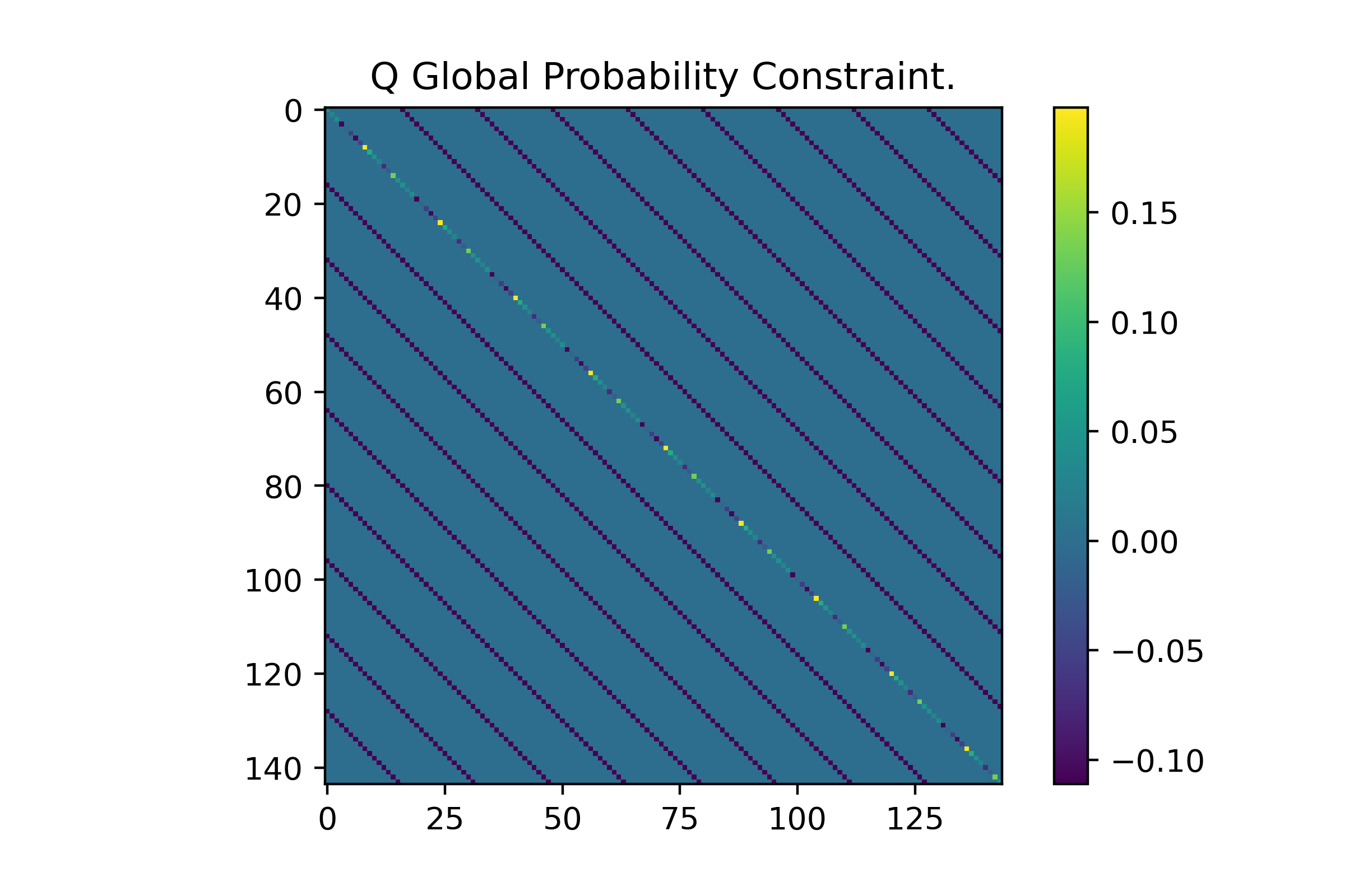
\[A = B(1 - 2{\sigma}_k(NN))\]I have arbitrarily decided we can set B to 1 resulting Q matrix that might look like:
.png)
What this matrix shows is that, by activating any qubit of tile type k, we reward the annealer with a positive value. However, by activating a qubit of the same type in any other location on the map we penalize the annealer with a negative value. The reward for activating a specific tile type is for linear \(N\) activations while the penalty is quadratic \(N*N\). Activating the number of tiles resulting in the desired frequency yields the maximum value of this function.
Now the optimal solution to our QUBO function is one where tile k only occurs with frequency \({\sigma}_k\)! This is close to a complete solution for procgen WFC, but it’s missing a very specific degree of control necessary for game development. In our dungeon example we need at least 1 entrance for our player to enter through and we may want to control where that entrance is placed by seeding that tile. The thought process for my proposed solution is as follows. For tile space [0, 0] we have the set of qubits:
\[\sum_{k=1}^{16}\sum_{k'=1}^{16}x_kx_{k'}a_{kk'}\]We also have the qubits corresponding to all cross activations:
\[\sum_{k=1}^{16}\sum_{j=17}^{NN}x_kx_ja_{kj}\]Where \(j\) spans all remaining cross-coefficients. If we want to seed the first tile with a dungeon entrance (tile # 3), then we end up with a vector
v = [0, 0, 0, 1, 0, 0, 0, 0, 0, 0, 0, 0, 0, 0, 0, 0]
Now all cross activation terms take on their seeded values, so for the first qubit we get:
\[x_1x_ja_{1j} = (0)x_ja_{1j} = (0)x_j^2a_{1j}\]and the third qubit
\[x_3x_ja_{3j} = (1)x_ja_{3j} = (1)x_j^2a_{3j}\]Once again, since a binary variable’s first order term is equal to its second order term, these can be added to the self activation coefficients of our remaining variables. Therefore, seeding a tile will only affect the weight along the diagonal. We now have 4 constraints in our Q matrix:
1) \(Q_{oneHot}\)
2) \(Q_{legal}\)
3) \(Q_{\sigma}\)
4) \(Q_{seeded}\)
With this we can generate a tile map where the annealer will choose only a single tile per grid space, the chosen tile will connect legally to its neighbors, each tile type will occur as close to a specified number of times as possible, and any grid space on the map can be seeded. This is very cool in my opinion and potentially very powerful. In m y opinion classical WFC is limited because it places tiles sequentially which will always pose a bottleneck. And while it’s remarkably simple to implement it’s also incredibly tricky to fix any incorrectly generated maps. QUBOs that are run on an annealer are free of both these problems because they find guaranteed correct solutions to complex problems extremely quickly!
Problems with QUBOs
HOWEVER, the tradeoffs are immense. From here on out is a discussion on the limitations of the QUBO and how they affect the procgen WFC solution shown so far. The main points are:
1) memory limitations 2) Randomness
The first of these problems is a modern hurdle for all quantum computers. The second of these problems stems from my inability to access a digital annealer at the moment. Either way, as with everything written so far, all comments, criticisms, suggestions, and collaborations are welcome!
1) Memory
The first and most immediate bottleneck with quantum hardware today is how limited it is by memory. A qubit is analogous to an actual bit, and a cutting edge annealer may only have access to around ~5k qubits. Our dungeon problem was building an [8 x 8] map with 16 tile types. This uses 1024 qubits. We clearly will not be generating a Minecraft sized world with this limited number of variables. We could generate a map of size [17 x 17] using 4624 qubits, but even then we aren’t exactly using a wide array of tile types. Now this isn’t necessarily a problem and it’s definitely not insurmountable. For instance it may not be as restrictive as we might think, after all, Into the Breach takes place on an [8 x 8] grid and those maps provide an immense amount of gameplay complexity. But what if we want to build something along the lines of one of the 2D Zelda maps? We could formulate this as a chunk generation problem, build 1000 [8 x 8] grids, and stitch them together to make an [800 x 800] sized map. Running these problems on an annealer is fast enough that 1000 solutions is still remarkably quick (and way faster than you could run traditional WFC). The question that remains is: How do you make a compelling world one [8 x 8] chunk at a time? (Spoiler I think I might use TF-IDF which comes from information theory and is used in document analysis)
2) Randomness
The point of WFC is to procedurally generate a different map every time you run the algorithm. An annealer solves a given QUBO problem. The annealer will therefore return the same solution each time if that solution is the most singularly optimal of all possible combinations. This is not random and not satisfactory for our intentions. Conversely, if two solutions are both globally optimal, the annealer should return one of the two randomly. A QUBO to demonstrate this would be:
\[Q = \begin{bmatrix}1 & -1\\ -1 & 1\end{bmatrix}\]Since either [1, 0] or [0, 1] are optimal the annealer should randomly activate either of the two qubits. I can’t test this however since I don’t have access to run time on an annealer >:( This potential randomness is important to know because depending on how you set up the constraints for a QUBO, any of the “legally placed solutions” should be optimal. The annealer should therefore return a random map. Since I am not a quantum physicist though and don’t actually know what that potential randomness will look like, is it normally distributed, is it true random? I DON’T KNOW WHY DID THEY REMOVE THE FREE ANNEALER ACCESS (I get why but I want to make silly game stuff).